Introduction

One of the most popular FIRE investment portfolios is the Boglehead Three-Fund Portfolio. Countless countless countless articles have been written on what this is and how to do it and so I don’t intend to contribute to that vast sea of articles.

Instead, I wanted to do a little projection to see how this might perform into the future. Yes, yes, I know I cautioned against using simulations (and why you shouldn’t get tricked by investment companies who use them to impress us) but I did caveat at the end that simulations can be helpful! They just shouldn’t be taken as the gospel truth. And so with that, my own simulation… ( as always, the code for the projections will be available at the end)

Portfolio Simulation

In true Boglehead’s fashion, I decided to simulate based on the traditional three-fund scenario. The traditional three components of the Bogleheads’ fund have been: International ETF, Local ETF, and Bonds. In following that, the funds I chose were:

IWDA — World ETF domiciled in Ireland to save on withholding taxes (yes, those really DO eat up your gains)
ES3 — Singapore Exchange ETF (just to get that little bit of local exposure)
A35 — Singapore Bonds (yawn, I’m so young I really don’t need bonds in my portfolio)

Simulation Parameters

In order to project future returns, I used a traditional Monte Carlo simulation. I had three portfolios of different weights and ran 1000 simulations on each portfolio. I know, very cool — but again, keep in mind that simulations are a helpful measure but NOT the truth.

In order to get the parameters for the projected returns of each portfolio, I used Yahoo Finance and gathered all the historical data from each of these three funds. I then calculated their monthly average return and standard deviation and used these in the Monte Carlo simulation.

As a quick visual tl;dr, these were the results of the simulations of the portfolios:

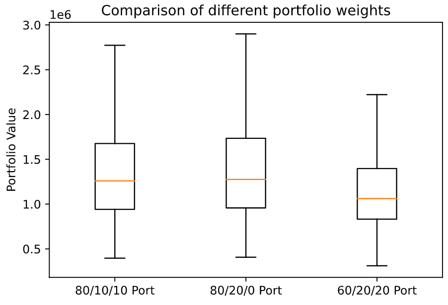
As you can see, the portfolios all had similar medians. The 80/20/0 portfolio (consisting of just equities and no bonds) evidently had a higher maximum value. However, the minimum value was about the same as the rest and the median was basically the same too.

So, that’s basically it if you were just interested in the overall comparisons. This (kinda) shows that you can basically go with whatever your heart desires. Want the possibility of more returns? 100% Equities it is! Want less volatility? Throw in some bonds! Because the returns (at least according to these very fallible simulations) are roughly the same.

Stick around for some pretty graphs!

80/10/10 Portfolio

The recommended portfolio — a good hearty chunk in the US/International market, some in your local equities, and some in bonds

80/20/0 Portfolio

Ah, someone who likes to live dangerously (basically me). All equities — who cares about bonds!

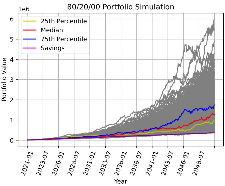
As you can see, slightly better returns than the 80/10/10 portfolio. But honestly not that much better.

60/20/20 Portfolio

I get it — you like to play it safe in life. Don’t dip your toes so much into those troubled US/International Equities waters. Chill in the SGX (nothing ever happens) and Bonds market.

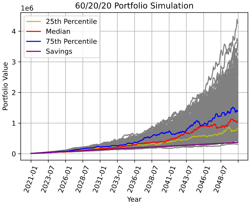
But guess what? You didn’t do half bad either! Just around $200,000 less but that ain’t too bad for reduced volatility.

Conclusion

So there we have it — a crystal ball into the future of using Monte Carlo simulations. I jest, we have (at best) a good rough approximation of what kind of returns we could expect to see.

Baring an economic meltdown, I think the biggest takeaway from these simulations are that investing consistently outperforms savings! So, even if you happened to fall into the 25th percentile, each scenario still gave you at least a 2X higher return than just stuffing your money under your pillow! So go out there and invest! And don’t be worried about being the worst investor in the world (and always investing just before a market crash) — you’ll still do well!

Code!

import random
import numpy as np
import matplotlib.pyplot as plt
import scipy.stats as stats
import pandas as pd
import math
import datetime
from dateutil.relativedelta import relativedelta

#set simulation start date
start_date = datetime.date(2021, 1, 1)
test_duration = 30
simulations = 1000

#create function to estimate returns for ETF using mean and std deviation
def EstimateReturns(initial_invest, expected_returns, std_dev, start_date, duration, monthly_con):
    final_money = []
    monthcount = []
        
     
    for month in range(duration*12):
        this_return = np.random.normal(expected_returns,std_dev)
        final_money.append(initial_invest)
        initial_invest = (initial_invest * (1+this_return)) + monthly_con
        a_date = (start_date + relativedelta(months=month))
        monthcount.append(a_date.strftime('%Y-%m'))  
    
    d = {'Date' : monthcount, 'Available Funds' : final_money}
    df = pd.DataFrame(data = d)
    final_funds.append(final_money[-1])
    return(df)
  
monthcount = []

for month in range(test_duration*12):
    a_date = (start_date + relativedelta(months=month))
    monthcount.append(a_date.strftime('%Y-%m')) 

tdf = pd.DataFrame({"Date" : monthcount}) 

# set portfolio weights - change this to try different weights!
weights = np.zeros(3)
weights[0] = 0.8
weights[1] = 0.2
weights[2] = 0.0
  
final_funds = []

# simulation across all three portfolios
for i in range(simulations):
    Stock1 = EstimateReturns(10000, 0.00685, 0.034, datetime.date(2021, 1, 1), test_duration, 1000)
    Stock2 = EstimateReturns(10000, 0.00109, 0.0509, datetime.date(2021, 1, 1), test_duration, 1000)
    Stock3 = EstimateReturns(10000, 0.0015, 0.0184, datetime.date(2021, 1, 1), test_duration, 1000)
    Stocks_total = pd.merge(Stock1,Stock2,how='left',on='Date')
    Stocks_total = pd.merge(Stocks_total,Stock3,how='left',on='Date')
    Stocks_total = Stocks_total.rename(columns={"Available Funds_x" : "SP500", "Available Funds_y" : "STI", "Available Funds" : "EIMI"})
    Stocks_total['Portfolio_Value {}'.format(i)] = Stocks_total['SP500']*weights[0] + Stocks_total['STI']*weights[1] + Stocks_total['EIMI']*weights[2]
    tdf = pd.merge(tdf,Stocks_total[['Date','Portfolio_Value {}'.format(i)]],on='Date', how='left')

 # transpose for easier graphing 
tryy = tdf.T
 
# create labelling for graph
bp3 = tryy.iloc[1:,-1].tolist() 
labels = ['80/10/10 Portfolio','80/20/0 Portfolio']

my_dict = {'80/10/10 Port': bp1, '80/20/0 Port': bp2, '60/20/20 Port': bp3}
 
# plot overall diagram (box and whiskers plot)
fig, ax = plt.subplots()
ax.boxplot(my_dict.values(), showfliers=False)
ax.set_xticklabels(my_dict.keys())
plt.ylabel("Portfolio Value")
plt.title("Comparison of different portfolio weights")
 
# Generate the names of the 25th, Median, and 75th perc portfolios
quantiles = []
for i in [0.25,0.5,0.75]:
    indx = str(tryy[tryy[tryy.shape[1]-1]==float(tryy.iloc[1:,tryy.shape[1]-1].quantile([i], interpolation = 'higher'))].index.tolist()).strip("[], '")
    quantiles.append(indx)

color=['y','r','b']
lab=['25th Percentile', 'Median', '75th Percentile']
 

monthcount = []

for month in range(test_duration*12):
    a_date = (start_date + relativedelta(months=month))
    monthcount.append(a_date.strftime('%Y-%m')) 

tdff = pd.DataFrame({"Date" : monthcount}) 

final_money = []
monthcount = []
initial_invest = 10000

for month in range(test_duration*12):
    final_money.append(initial_invest)
    initial_invest = (initial_invest + 1000)
    a_date = (start_date + relativedelta(months=month))
    monthcount.append(a_date.strftime('%Y-%m'))  

d = {'Date' : monthcount, 'Available Funds' : final_money}
savings = pd.DataFrame(data = d)
savings
savings = pd.merge(tdff,savings,on='Date', how='left')
 

# Graph the final portfolios
labels = []
fig, ax = plt.subplots()
for i in range(1, len(tryy)):
    ax.plot(tryy.iloc[0,:], tryy.iloc[i,:], color='grey')
    labels.append("Portfolio No: {}".format(i))

for i in range(0,len(quantiles)): 
    ax.plot(tryy.iloc[0,:], tryy.loc[quantiles[i],:], color=color[i], label=lab[i])

ax.plot(savings.iloc[:,0], savings['Available Funds'], color='purple', label="Savings")
ax.xaxis.set_major_locator(plt.MaxNLocator(15))
plt.setp(ax.get_xticklabels(), rotation=70, ha="center")
plt.ylabel("Portfolio Value")
plt.xlabel("Year")
plt.title("60/20/20 Portfolio Simulation")
plt.grid()
leg = ax.legend()

print("The median portfolio value is: {}".format(round(tryy.iloc[1:,tryy.shape[1]-1].median(),2)))
print("The 75th percentile portfolio value is: {}".format(round(float(tryy.iloc[1:,tryy.shape[1]-1].quantile([0.75])),2)))
print("The 25th percentile portfolio value is: {}".format(round(float(tryy.iloc[1:,tryy.shape[1]-1].quantile([0.25])),2)))
print("The savings portfolio value is: {}".format(round(float(savings.iloc[-1,1]))))