
Using Pandas to implement Stop Losses and Take Profits for trading strategy backtests
Introduction
Backtesting is an important part of any strategy. An essential part of most strategies is having a Stop Loss and a Take Profit. In Python, there are a myriad of backtesting options available to you that allow for this but sometimes simple is better. Today, we’re going to look at how one can implement a Stop Loss and Take Profit using pandas before then using bt to run the full backtest.
Contents
- Overview of bt
- Using pandas to implement Stop Loss and Take Profits
- Setting weights for bt
- Running the backtest
1. Overview of bt
bt is a “flexible backtesting” framework for Python that is modular. What this means is that bt has a number of algorithms that are pre-built that one can literally “plug-and-play” with to get different backtesting outcomes. One of the core algo modules in bt is the weighTarget algo. This algo essentially rebalances a portfolio again and again in order to match the weight given to a particular stock position. For instance, this is a table of weights below. When the target weight (TW) is 0.33, the algo will invest 0.33 of available cash into the position, -0.33 will make it go short, and 0 will cause it to exit the position.
| NFLX | AAPL | GOOG | |
|---|---|---|---|
| 2015-03-20 00:00:00+00:00 | -0.333333 | 0.000000 | 0.000000 |
| 2015-03-23 00:00:00+00:00 | -0.333333 | 0.000000 | 0.000000 |
| 2015-03-24 00:00:00+00:00 | -0.333333 | 0.000000 | 0.000000 |
| 2015-03-25 00:00:00+00:00 | -0.333333 | -0.333333 | 0.000000 |
| 2015-03-26 00:00:00+00:00 | -0.333333 | -0.333333 | 0.000000 |
| ... | ... | ... | ... |
| 2020-10-05 00:00:00+00:00 | 0.333333 | 0.333333 | 0.333333 |
| 2020-10-06 00:00:00+00:00 | 0.333333 | 0.333333 | 0.333333 |
| 2020-10-07 00:00:00+00:00 | 0.333333 | 0.333333 | 0.333333 |
| 2020-10-08 00:00:00+00:00 | 0.333333 | 0.333333 | 0.333333 |
| 2020-10-09 00:00:00+00:00 | 0.333333 | 0.333333 | 0.333333 |
1401 rows × 3 columns
This makes backtesting very simple because we just have to generate a dataframe of weights and bt will run through the weights. What makes it challenging then is setting the weights… and that’s where pandas comes into play!
2. Using pandas to prepare the weights (with SL and TP implementation!)
We will be implementing a super simple (AND super non-profitable) strategy that makes use of 2 popular technical indicators - the Relative Strength Indicator and the MACD. We will be setting the Stop Losses (SL) and Take Profits (TP) as fixed percentages of the price (note: NOT a trailing stop, just a fixed stop loss)
To make things clear, the logic of the strategy is as follows:
-
If RSI > 50 and MACD > 0: Buy Signal
-
If RSI < 50 and MACD < 0: Sell Signal
-
Once we enter a position, the SL will be 0.97x(entry price) and the TP will be 1.5x(entry price).
import pandas as pd
from tiingo import TiingoClient # for historical data
### for my technical indicators
from ta.momentum import RSIIndicator, stoch
from ta.trend import MACD as md
I used Tiingo to get my historical data but you can use your data provider of choice! For this backtest, we are only going to use three stocks (but once you implement this, you can use as many stocks as you want)
client = TiingoClient({'api_key' : 'SECRET_API_KEY'})

datalist = ['NFLX', 'AAPL', 'GOOG']

data = client.get_dataframe(datalist,
                                    metric_name='adjClose',
                                      frequency='daily',
                                      startDate='2015-02-02',
                                      endDate='2020-10-10')
Once we have our data, we now need to write a function that would allow us to set our target weights (as per the dataframe shown previously). The code may seem long and tricky but its really simple once you think about it.
def RSI_base(data,ticker):
    MACD = md(close=data[ticker])
    data["MACD_diff"] = MACD.macd_diff()
    RSI = RSIIndicator(close=data[ticker])
    data["RSI"] = RSI.rsi()
    data["Buy_Signal"] = 0
    data["Sell_Signal"] = 0
    data["SL"] = 0
    data["TP"] = 0
    data["Pos"] = 0
    data["TW"] = 0.0
The first thing we do is initialize our indicators and create another column to input their values. Next, we create a number of columns that will allow us to keep track of our positions - we have our buy_signal, our sell_signal, our SL and TP, a column to show whether we are in a Position or not, and finally our target weights (TW).
    for i in range(0,len(data)):
        if data["Pos"][i-1] == 0:
            if data["RSI"].iloc[i] > 50 and data["MACD_diff"][i] > 0 and (data["Pos"][i] == 0):
                data["Buy_Signal"][i] = 1
                data["Pos"][i] = 1
                data["SL"][i] = (data[ticker][i]*0.97)
                data["TP"][i] = (data[ticker][i]*1.5)
            elif data["RSI"].iloc[i] < 50 and data["MACD_diff"][i] < 0 and (data["Pos"][i] == 0):
                data["Buy_Signal"][i] = 1
                data["Pos"][i] = -1
                data["SL"][i] = (data[ticker][i]*1.03)
                data["TP"][i] = (data[ticker][i]*0.95)
            else:
                data["Buy_Signal"][i] = 0
                data["Pos"][i] = 0
The next section of the function starts with asking if there is a position open. We use [i-1] as a reference because we need to refer to the row above in order to determine if a position is currently open. If there is no position open, we then issue our buy and sell orders! (I’m aware that selling short should technically be a ‘sell signal’ but for simplicity, as long as we’re opening a new position, we call it a ‘buy_signal’)
We then set our positions to either 1 (for long positions) or -1 (for short positions). We calculate our SL and TP and also set those.
Of course, if there is no signal, we leave position as 0 (for no position)
        elif data["Pos"][i-1] == 1:
            data["SL"][i] = data["SL"][i-1]
            data["TP"][i] = data["TP"][i-1]
            if (data[ticker][i] > data["SL"][i-1]) or (data[ticker][i] < data["TP"][i-1]):
                data["Pos"][i] = 1
            if (data[ticker][i] < data["SL"][i]) or (data[ticker][i] > data["TP"][i-1]):
                data["Pos"][i] = 0
                data["Sell_Signal"][i] = 1

        elif data["Pos"][i-1] == -1:
            data["SL"][i] = data["SL"][i-1]
            data["TP"][i] = data["TP"][i-1]
            if (data[ticker][i] < data["SL"][i-1]) or (data[ticker][i] > data["TP"][i-1]):
                data["Pos"][i] = -1
            if (data[ticker][i] > data["SL"][i]) or (data[ticker][i] < data["TP"][i-1]):
                data["Pos"][i] = 0
                data["Sell_Signal"][i] = 1
The next block is important because it sets the logic that allows the SL and TP to be used. It checks if the position is a long or short position and then sets the current SL and TP to the preceeding one. This allows the SL and TP to be persistent. After setting the SL and TP for the current line, we check if the price of the ticker is below or above the SL and TP (respectively, for long positions and vice versa for short positions).
If the price has crossed the SL or TP, we set our positions to 0 (i.e. exit our positions) and then set the sell_signal to 1 (indicating a sell)
    for i in range(len(data)):
        if (data["Pos"][i] == 1):
            data["TW"][i] = 1/len(datalist)
        elif (data["Pos"][i] == -1):
            data["TW"][i] = -(1/len(datalist))
        else:
            data["TW"][i] = 0

    weights = data["TW"]

    return weights
Whew! We’re at the end of the function! Finally, in the last part of the function, we calculate the TW for our positions. Its simply a matter of referring to our positions column - if the position is a long column, we set the weight to 1/len(datalist) and if short the negative of that (under the assumption we are going to balance the portfolio equally). Of coure, if no position is open, we set the TW to 0 (which will also trigger a close of the position if there was previously an open position).
3. Settings weights for bt
The next part is relatively simple. With this function, we get a pandas.series containing the weights for a particular ticker. We create a for loop to loop through all the tickers in our datalist and then assign the weights series to temp. We also need to rename it to the ticker name (this is to allow bt to match the weights to the data). This is how we get the df shown at the start of the article.
I also clean up the “data” dataframe, removing all the unnecessary columns that we created and simply retaining the stock price data.
df = pd.DataFrame()

for i in datalist:
    temp = RSI_base(data,i)
    temp = temp.rename(i)
    df = pd.concat([df,temp],axis=1)

data = data[['NFLX', 'AAPL', 'GOOG']]
4. Running the backtest
And… with that, the hard part is over! All that’s left to do is to feed this table of weights to bt and run our backtest. I won’t be going into detail about bt here because that’s really not the focus of the article but drop me a note if you want to chat more about bt/have an article about it!
import bt
import matplotlib.pyplot as plt
import numpy as np
#create strategy
crosses = bt.Strategy('Test1', [bt.algos.WeighTarget(df),
bt.algos.Rebalance()])
#create benchmark of buy-and-hold
long_only = bt.Strategy('Benchmark', [bt.algos.RunOnce(),
bt.algos.SelectAll(),
bt.algos.WeighEqually(),
bt.algos.Rebalance()])
#set backtests and commissions
t = bt.Backtest(crosses,data,commissions=lambda q, p: max(1, abs(q) * 0.05))
s = bt.Backtest(long_only, data,commissions=lambda q, p: max(1, abs(q) * 0.05))
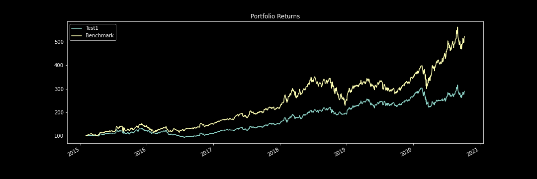
report = bt.run(t,s)
plt.title("Portfolio Returns")
report.plot()
Test1
0% [############################# ] 100% | ETA: 00:00:00Benchmark
0% [############################# ] 100% | ETA: 00:00:00
report.set_riskfree_rate(0.001)
report.display()
Stat                 Test1       Benchmark
-------------------  ----------  -----------
Start                2015-02-01  2015-02-01
End                  2020-10-09  2020-10-09
Risk-free rate       0.10%       0.10%

Total Return         189.47%     424.46%
Daily Sharpe         0.93        1.14
Daily Sortino        1.49        1.88
CAGR                 20.55%      33.83%
Max Drawdown         -30.97%     -34.69%
Calmar Ratio         0.66        0.98

MTD                  4.01%       5.03%
3m                   5.45%       9.00%
6m                   28.16%      48.02%
YTD                  9.41%       52.04%
1Y                   27.37%      83.19%
3Y (ann.)            26.36%      35.31%
5Y (ann.)            20.09%      31.69%
10Y (ann.)           20.55%      33.83%
Since Incep. (ann.)  20.55%      33.83%

Daily Sharpe         0.93        1.14
Daily Sortino        1.49        1.88
Daily Mean (ann.)    21.26%      33.40%
Daily Vol (ann.)     22.69%      29.17%
Daily Skew           -0.27       -0.14
Daily Kurt           4.06        4.07
Best Day             7.61%       8.99%
Worst Day            -8.00%      -11.56%

Monthly Sharpe       0.96        1.24
Monthly Sortino      1.83        2.73
Monthly Mean (ann.)  21.29%      31.42%
Monthly Vol (ann.)   22.02%      25.26%
Monthly Skew         -0.31       -0.00
Monthly Kurt         0.26        -0.17
Best Month           15.78%      22.37%
Worst Month          -16.93%     -13.99%

Yearly Sharpe        0.98        1.63
Yearly Sortino       4.38        inf
Yearly Mean          20.70%      31.72%
Yearly Vol           21.11%      19.39%
Yearly Skew          -0.90       -0.37
Yearly Kurt          -0.65       -2.20
Best Year            38.74%      52.04%
Worst Year           -10.52%     6.90%

Avg. Drawdown        -3.68%      -3.71%
Avg. Drawdown Days   28.66       23.18
Avg. Up Month        5.71%       6.86%
Avg. Down Month      -4.58%      -5.67%
Win Year %           80.00%      100.00%
Win 12m %            82.76%      86.21%
So, obviously NOT a market-beating strategy but not too terrible if I do say so myself.
Conclusion
In this article, we saw how we can work within pandas to create a strategy that has bracket orders of SL and TP. We then used bt to run the strategy. That’s all for now. Thanks for reading and let me know if you have any questions!