
Using a Monte Carlo simulation to determine the Fair Value of a stock
Introduction
One of the most popular ways to value a company is using a model known as the Discounted Cash Flow Model. This model attempts to find the intrinsic value of a company by projecting its future cash flows and then discounting it. This is typically done using an excel spreadsheet and is relatively simple (just requiring a little bit of math and some manual work to find the financial information of a company). In this article, we’re going to explore how we can easily automate this in Python (both the calculation as well as the pulling of financial data!), adding in a monte carlo simulation to try to get a better range of intrinsic value calculations.
Pulling Financial Information
The first step is to pull financial data. We are using the FundamentalAnalysis package which allows us to access data from FinancialModelingPrep (FMP). In order to use FMP, you need to get a free API key, which you can get here. The first step is really simple - all we’re doing is downloading the Cash Flow statement, the Income Statement, and the Balance Sheet via FMP’s API.
import FundamentalAnalysis as fa
import pandas as pd
import matplotlib.pyplot as plt
import numpy as np
import yfinance as yf

ticker = "AMD" #ticker name
api = "384de232a09606f8ff4de3489690dc4c" #api key

#get company profile for beta calculation and marketcap
profile = fa.profile(ticker, api)
quote = fa.quote(ticker, api)

#FMP gives the dates reversed and hence the need for the .iloc in all the data calls
#get the cash flow, income statement, and balance sheet
cf = fa.cash_flow_statement(ticker, api).iloc[:,::-1]
ins = fa.income_statement(ticker, api).iloc[:,::-1]
bs = fa.balance_sheet_statement(ticker, api).iloc[:,::-1]

year = "2019" #set year
FMP returns the statements in descending order which we don’t want. Hence, there’s a need to use the .iloc[:,::-1] to flip it around.
DCF Valuation
There are three main parts to doing a DCF valuation.
1. Project Future Cash Flow.
There are many ways to do this and the most direct would be to just find the mean growth of cash flow and project it forward. However, another way to do it would be to project revenue first. From revenue, we can then project net income, and finally project free cash flow. To do this, we would need revenue/income ratios (i.e. income margin) and also free cash flow/revenue ratios. Being conservative, we then take the lowest positive number of the income margin ratios and free cash flow/revenue ratios.
Below, we first gather the last 5 years of data that we have, and then derive our estimates for revenue change, income margin, and fcf/revenue. As you can see, we use .min() to be conservative. Since we want to do a Monte Carlo simulation, we need both the mean and the standard deviation for our revenue growth. For our later simulation, we will need the risk free rate of return. This is usually assumed to be the returns of the 10-year treasury bonds and we use yfinance to obtain that
dcf_proj = pd.DataFrame({
    "revenue" : ins.loc["revenue"],
    "netincome" : cf.loc["netIncome"],
    "freecash" : cf.loc["freeCashFlow"]
}).transpose()

dcf_proj.loc["incomeMargin"] = dcf_proj.loc["revenue"]/dcf_proj.loc["netincome"]
dcf_proj.loc["FCFr"] = dcf_proj.loc["revenue"]/dcf_proj.loc["freecash"]
rev_change_mean = ins.loc["revenue"].pct_change().mean()
rev_change_stdd = ins.loc["revenue"].pct_change().std()
margin_change = dcf_proj.loc["incomeMargin", dcf_proj.loc["incomeMargin"] > 0].min()
fcf_change = dcf_proj.loc["FCFr", dcf_proj.loc["FCFr"] > 0].min()

tnx = yf.Ticker("^TNX") #use yfinance to get the 10yr treasury bond return
rfr = tnx.info["previousClose"] #use previousclose to estimate rfr

dcf_proj
| 2015 | 2016 | 2017 | 2018 | 2019 | |
|---|---|---|---|---|---|
| revenue | 3991000000 | 4272000000 | 5253000000 | 6475000000 | 6731000000 |
| netincome | -660000000 | -497000000 | -33000000 | 337000000 | 341000000 |
| freecash | -322000000 | 13000000 | -101000000 | -129000000 | 276000000 |
| incomeMargin | -6.04697 | -8.59557 | -159.182 | 19.2136 | 19.739 |
| FCFr | -12.3944 | 328.615 | -52.0099 | -50.1938 | 24.3877 |
We continue with our projections of future cash flows below. Using the estimations we got above, we plug these into a 5-period for loop to obtain our forward estimations. We use np.random.normal() with the mean and standard deviation of the revenue change obtained above. The code is then plugged into a parent for loop in order to run the simulation.
startrev = dcf_proj.loc["revenue",year] #get the starting revenue

allFVs = [] #create a list to store FV values

for p in range(10000): #run the simulation 10000 times
    #creating projections for a 5 year dcf model
    Fiveyrev = []
    Fiveyinc = []
    Fiveyfcf = []
    for i in range(5):
        startrev = startrev*(1+np.random.normal(loc=rev_change_mean, scale=rev_change_stdd))
        neti = startrev*(margin_change/100)
        fcf = neti*(fcf_change/100)
        Fiveyrev.append(startrev)
        Fiveyinc.append(neti)
        Fiveyfcf.append(fcf)
2. Discount Projected Cash Flow
We now have our projected cash flows but need to discount them to find the Present Value (PV). This is because $100 today will not have the same value as $100 in the future. Hence, we need to discount the future value of the cash (i.e. reduce its value to what it would be worth today). Again, there are many ways to do this but one way to get the discount rate is to use the Weighted Average Cost of Capital (WACC).

The equation seems really scary at first but its really basic math. Essentially, we find the cost of the firm’s debt and the cost of the firm’s equity and then weigh them (hence the word “weighted”). If you want to go into greater depth as to how this is done, this video is particularly helpful. The code is basically a translation of the equation. We find the past 5 years of Wacc in order to calculate the standard deviation.
beta = profile.loc["beta"] #get beta of stock from stock profile
mktCap = quote.loc["marketCap"] #market cap of stock
totdebt = bs.loc["totalDebt",year] #total debt
sharesOut = quote.loc["sharesOutstanding"]
pg = 0.025 #perpetural growth

wacklist = []
for i,d in enumerate(["2015","2016","2017","2018","2019"]):
    Rd = ins.loc["interestExpense", d]/totdebt*(1-(ins.loc["incomeTaxExpense",d]/ins.loc["incomeBeforeTax",d]))
    Re = rfr + (beta*(10 - rfr))
    wacc = float(((Rd)*(totdebt/(mktCap + totdebt)) + (Re)*(1-(totdebt/(mktCap + totdebt))))/100)
    wacklist.append(Wacc)

wacc_stdd = np.std(wacklist)
We also need to find “Terminal Value” which is the value of the company beyond the 5 years that we are projecting. This requires an estimation of the perpetual growth rate of the company. We typically use 2.5% because this is lower than the growth rate of the economy (and it cannot be higher than the economy unless we think that one day this company will be LARGER than the entire economy)
For the discount value, we also use np.random.normal(), setting the mean as the current WACC and the standard deviation as the std dev. of the last 5 years of WACC.
# continuing the for loop...

    DV = np.random.normal(loc=wacc, scale=wacc_stdd)

    TV = float(((Fiveyfcf[-1]*(1+pg))/(DV - pg))) #Obtain Terminal value
    Fiveyfcf.append(TV)
After obtaining the Terminal Value and calculating the Discount Value, we now have to apply the discount to all the projected cash flows. The discount equation is as follow:
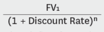
We go through the list of projected cash flows and apply the discount formula to them
    Fiveyfcfdisc = []

    for i,d in enumerate(Fiveyfcf): #apply discount formula to all projected cash flows
        disc = float(Fiveyfcf[i]) * (1+DV)**(1+i)
        Fiveyfcfdisc.append(disc)
3. Calculating Net Present Value and Fair Value
And… we’re almost done! All that’s left to do is calculate the Net Present Value by summing up the discounted cash flows. And then dividing by the total number of shares issued by the company. We then append the calculated Fair value to a list so that we can keep track of all the calculated FVs in our simulation.
    FV = round(float(float(sum(Fiveyfcfdisc))/sharesOut),2) #divide NPV by shares

    allFVs.append(FV) #add to the list
With that, we have our simulated output of Fair Values! We can then work with these outputs by, for instance, plotting them in a histogram and determining the median Fair Value.
import matplotlib.pyplot as plt

plt.hist(allFVs, density=True, color="darkblue")
plt.title("Monte Carlo Plot of Fair Value")
plt.xlabel("Fair Value")
plt.ylabel("Count")

print("Median Fair Value: {}".format(np.median(allFVs)))
Median Fair Value: 15.17

Conclusion
Thanks for reading! This was a simple guide to how one can use a Monte Carlo simulation in order to ascertain the range of Fair Value when performing stock valuation using a Discounted Cash Flow model.